Design Of Experiment

 Week 13 💗

This week, we learnt how to do Design of experiment, or DOE for short. In this blog, I would be doing a Full Factorial analysis and a Fractional Factorial analysis on a case study that was given to me. Since I am the CFO of my group for the final group project, I am tasked to do the second case study. 

Background on Case 2:

What could be simpler than making microwave popcorn? Unfortunately, as everyone who has ever made popcorn knows, it’s nearly impossible to get every kernel of corn to pop. Often a considerable number of inedible “bullets” (unpopped kernels) remain at the botoom of the bag. What causes this loss of popcorn yiled?

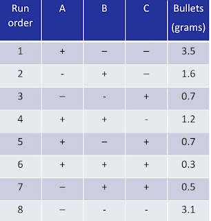
 In this case study, three factors were identified: 

1. Diameter of bowls to contain the corn, 10 cm and 15 cm

 2. Microwaving time, 4 minutes and 6 minutes 

3. Power setting of microwave, 75% and 100%

 8 runs were performed with 100 grams of corn used in every experiments and the measured variable is the amount of “bullets” formed in grams and data collected are shown below: 

Factor A= diameter 

Factor B= microwaving time 

Factor C= power 

Full Factorial Analysis  👀

Using the template of excel that was given to us by our lecturer, 

From the graph, the factor that is the most significant is Factor C, as the gradient is the steepest among the other factors, while factor A is the least significant as the gradient is the lest steep. 

From the most significant to the least significant factor, 

Factor C> Factor B> Factor A

AxB

At low B, Average of low A= (3.1+0.7)/2= 1.9 (-)

At low B, Average of high A= (3.5+0.7)/2= 2.1 (+)

At low B, total effect of A= (2.1+1.9)/2= 0.2 (increase)

At high B, Average of low A= (1.6+0.5)= 1.05 (-)

At high B, Average of high A = (1.2+0.3)= 0.75 (+)

At high B, total effect of high A= (0.75-1.05)/2 = -0.3 (decrease)

From the graph of the interaction between A and B, there is an interaction between the two factors as the gradients for both the factors are different.

AxC

At low C, Average low A= (1.6+3.1)/2= 2.35 (-)

At low C, Average high A= (1.6+3.1)/2= 2.35 (+)

At low C, total effect of A= (2.35-2.35)= 0 (no effect)

At high C, Average of low A= (0.7+0.5)/2= 0.6 (-)

At high C, Average of high A= (0.7+0.3)/2= 0.5 (+)

At high C, total effect of A= (0.5-0.6)/2= 0.6 (decrease)

From the graph of the interaction between A and C, there is an interaction between the two factors as their gradients are very different. However, the interaction is small as the lines are almost parallel. 

BxC

At low C, Average of low B= (3.5+3.1)/2= 3.3 (-)

At low C, Average of high B= (1.6+1.2)/2= 1.4 (+)

At low C, total effect of B= (1.4-3.3)/2= -1.9 (Decrease)

At high C, Average of low B= (0.7+0.7)/2= 0.7 (-)

At high C, Average of high B= (0.3+0.5)/2= 0.4 (+)

At high C, total effect of B= (0.4-0.7)/2= -0.3 (Decrease)

From the graph of the interaction between B and C, the interaction between the two are very significant as the two lines on the graph are very different.  

Excel File: 

https://docs.google.com/spreadsheets/d/1e4VGxiydBlN6loP_8NN4Za12a28OYxNN/edit?usp=sharing&ouid=115367649934172105803&rtpof=true&sd=true

Fractional Factorial analysis:👀

A fractional factorial analysis is a shortened version of a full factorial, which makes it easier to see the significance of the different factors. 

Considering the statistical orthogonality, I would choose runs 1,4,6 and 7 for my fractional factorial. 

Using the excel template by my lecturer, 

From the fractional factorial,

The effects of each factor;

Diameter: 

When the diameter increases, the amount of bullets formed also increases.

Microwaving Time:

As the microwaving time increases, the amount of bullets formed also decreases.

Power:

As the power increases, the amount of bullets formed also decreases.

Conclusion: 

Factor C is still the most significant factor as it has the steepest gradient among all the other factors' gradient, while factor A is still the least significant factor due to it's gradient being the least steep. 

Reflection 💭🧠

After doing this case study, I do feel that I can understand DOE a lot better as when I first learnt about it I was a little confused. I feel that this would definitely come in handy when we have many different sets of data, and with this, it would be easier to analyze the data that we have collected. Hence, this would be especially useful when it comes to testing our prototype and in our final year project. 

Excel File:

https://docs.google.com/spreadsheets/d/1Chu2mi5DdED-ngLCmdF35SvCfjiEkl1R/edit?usp=sharing&ouid=115367649934172105803&rtpof=true&sd=true